Introduction

Beyblade has proven itself to be a strong-running franchise, spanning several TV series and toys. In the shows and on the boxes of said toys, there is an emphasis on the attributes of the beyblades: their Attack, Defense, and Stamina for each component that make up the beyblade. While the validity of these statistics can be questioned, one cannot help but wonder about the relationship between these three traits among the beyblades. In this post, I will focus on the Metal Fight subseries of beyblades, scraping their statistical information on the Metal Fight Beyblade wiki¹ and graphing the attributes against each other to determine the hypothetical optimal beyblade. In other words, I will walk through the process of obtaining these statistics and graphing the results.

Setup

I will first start by loading some necessary libraries, primarily consisting of tidyverse packages with a particular emphasis on purrr and ggplot2. Our main web-scraping tool will be rvest. Other libraries include ggthemes and gridExtra for plotting, as well as knitr, kableExtra, and flextable for table formatting. I construct a for-loop statement to test whether the packages have already been installed–if not, install it.²

libs <- c('tidyverse', 
          'rvest', 
          'magrittr', 
          'ggthemes', 
          'gridExtra', 
          'knitr',
          'kableExtra',
          'flextable')

for (i in libs) {
  
  if (!require(i, character.only = TRUE)) {
    
    install.packages(i)
    library(i, character.only = TRUE)
    
  }
  
}

Wiki Mining

To scrape the required Metal Fight beyblades, I refer to the Metal Fight BeyBlade wiki (https://mfbeyblade.fandom.com/wiki/Beyblades). Using rvest, I import the URL of the beyblades-list page; find the node that encases these beyblades in a list (the “ul” node); and make the appropriate text modifications, primarily filtering out blanks and splitting the beyblade names into a clean vector–that is, the beyblade names are initially inside a single element, so I split them out into a vector of names.

One interesting note: as of this writing, “Big Bang Pegasus” is misspelled as “Big Bang Pegasis” in its URL. I make this additional modification so that we can scrape this particular beyblade’s statistical information.

page <- 'https://mfbeyblade.fandom.com/wiki/Beyblades'

bbs <- read_html(page) %>%
  # List of Beyblades is...in a list.
  ## Find them in the list node.
  html_nodes("ul") %>% 
  # Convert to text.
  html_text() %>% 
  # Take out the tab separators.
  gsub('\t', '', .) %>% 
  # Filter out blanks
  subset(., . != '') %>% 
  # List of beyblade names is stuffed inside a single element.
  .[[11]] %>% 
  # Split by this separator.
  str_split('\n') %>% 
  # output is a list: convert to vector.
  .[[1]] %>% 
  # Filter out blanks.
  subset(., . != '') %>% 
  # URL hyperlinks have underscores.
  gsub(' ', '_', .) 

# Wiki link has spelling error for Big Bang Pegasus
bbs[bbs == 'Big_Bang_Pegasus'] <- 'Big_Bang_Pegasis' 

# For the get_stats function later.
beyblades <- data.frame(bb = bbs)

Once I have our vector of names, I note that the beyblade URLs in the wiki have a common naming scheme: https://mfbeyblade.fandom.com/wiki/[Beyblade Name]. As such, I prefix this pattern to each beyblade name I have obtained earlier. Next, I write a fairly complex function to take into account whether a beyblade page has multiple tables of information or no tables at all. Because the statistics are coded with asterisks instead of numbers, I have to count each asterisk to know the numeric power level of a particular trait (Attack, Defense, and Stamina). Additionally, because the statistics are for each component of the beyblade (i.e. the parts of the beyblade) rather than overall, I sum the traits to obtain a summary statistic for that particular trait (i.e. Total Attack Power across the components, Total Defense Power across the components, and Total Stamina Power across the components). Finally, I use map2_df from the purrr library within tidyverse to iterate over the URLs and beyblade names in parallel.

urls <- paste0('https://mfbeyblade.fandom.com/wiki/', beyblades$bb)

get_stats <- function(u, b) {
  
  # u = URL
  # b = Beyblade name
  
  # Get table of statistics
  stats <- read_html(u) %>%
    html_nodes('table') %>%
    html_table(fill = TRUE)
  
  
  # Element-checking
  if (length(stats) > 1)  {
    
    # First table might be the wikipedia side bar
    stats %<>% .[[2]] 
    
  } else if (length(stats) == 1) {
    
    stats %<>% .[[1]]
    
  } else {
    
    # Give a fake vector for the next type checking
    stats <- data.frame(x = 1:2) 
    
  }
  
  # Rename columns based on first row.
  names(stats) <- stats[1, ]
  
  # Select only the necessary rows.
  stats %<>%
    .[2:NROW(.), ]
  
  # Element-checking
  if (!'Attack' %in% names(stats)) {
    
    # If the beyblade doesn't have stats on the page,
    ## remove it from analysis.
    stats2 <- NULL
    
  } else {
    
    # The stats are labeled by stars (*).
    ## We need to convert them into numbers.
    stats[, c('Attack', 'Defense', 'Stamina')] %<>%
      map_df(~ gsub(' ', '', .x)) %>%
      map_df(~ nchar(.x))
    
    # Face top stats do not exist and
    ## should be removed.
    stats %<>%
      mutate(Beyblade = b) %>%
      slice(2:NROW(.))
    
    # Append Overall stats based on the sum.
    overall <- data.frame(Part = 'Overall',
                          Name = 'Overall',
                          Attack = sum(stats$Attack),
                          Defense = sum(stats$Defense),
                          Stamina = sum(stats$Stamina),
                          Beyblade = b,
                          stringsAsFactors = FALSE)
    
    stats2 <- bind_rows(stats, overall)
    
    stats2
    
  }
  
}


# Defensive check
get_stats_possibly <- possibly(get_stats, NA)

# By URL and beyblade, obtain the stats.
bbs <- map2_df(urls, beyblades$bb, get_stats_possibly) %>%
  # We only need the "Overall" stats.
  filter(Name == 'Overall') %>%
  # First two columns are now irrelevant.
  select(3:NCOL(.)) %>%
  # Reorder.
  select(Beyblade, everything())

The table below shows what the final dataset looks like.

flextable(bbs) %>% 
  set_caption(caption = 'Table 1: Overall Beyblade Statistics')

Results

To start plotting the results, I use a small-multiples approach³ to plot Attack against Defense, Attack against Stamina, and Defense against Stamina. For the following graphs, I like the more minimalistic approach of theme_light(): it’s simple, but adds a touch of detail that makes it stand out relative to theme_minimal(), I feel.

# Generalize the aesthetics, geometries, and theme.
plot_bbs <- function(data, y, x) {
  
    ggplot(data) + 
    aes_string(y = y, 
               x = x, 
               label = 'Beyblade') +
    geom_text(col = 'cyan4', 
              position = position_jitter()) + 
    geom_smooth(method = 'lm', 
                col = 'salmon', 
                se = FALSE,
                alpha = 0.5, 
                linetype = 2) + 
    labs(y = paste('Total', y),
         x = paste('Total', x)) +
    theme_light() + 
    theme(panel.grid.minor = element_blank(),
          panel.grid.major.x = element_blank())
  
}

# Small multiples
g1 <- plot_bbs(bbs, 'Attack', 'Defense')
g2 <- plot_bbs(bbs, 'Attack', 'Stamina')
g3 <- plot_bbs(bbs, 'Defense', 'Stamina')

# Arrange in a grid
grid.arrange(g1, g2, g3, nrow = 2, ncol = 2, 
             top = 'Fig. 1: Beyblade Statistics Comparisons')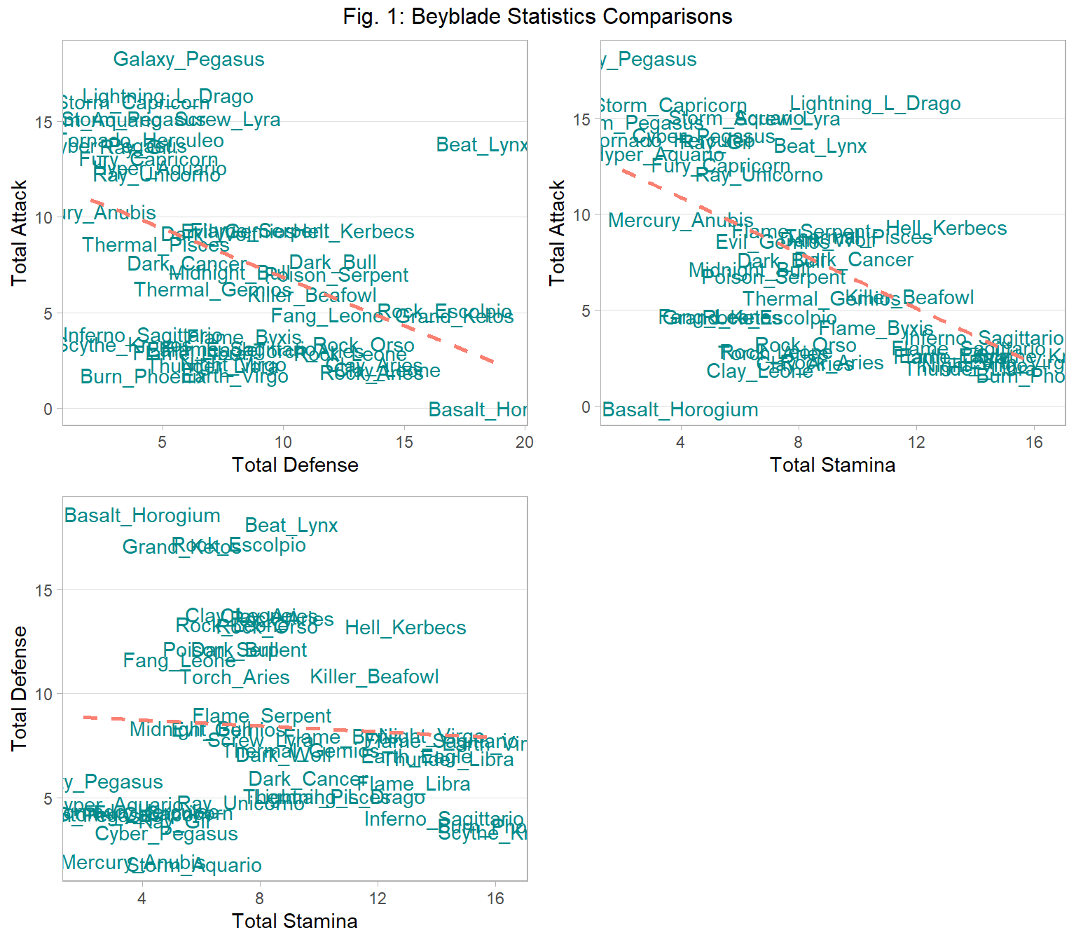

Based on Figure 1, there is a negative trend between Attack and Defense, as well as between Attack and Stamina–this finding implies that there exists a general trade-off between Attack and another trait. However, the relationship between Defense and Stamina is relatively flat, which may indicate that Defense is not correlated with Stamina.

Alternatively, we can set Stamina as the size input to have a single display of all the traits.

plot_bbs2 <- function(data) {
  
  ggplot(data) + 
    aes_string(y = 'Attack', 
               x = 'Defense',
               size = 'Stamina',
               label = 'Beyblade') +
    geom_text(col = 'cyan4', 
              position = position_jitter()) + 
    labs(y = 'Total Attack',
         x = 'Total Defense',
         size = 'Total Stamina',
         title = 'Fig. 2: Beyblade Statistics Comparisons (Alt. Display)'
         ) +
    theme_light() + 
    theme(panel.grid.minor = element_blank(),
          panel.grid.major.x = element_blank(),
          legend.position = 'bottom')
  
}

plot_bbs2(bbs)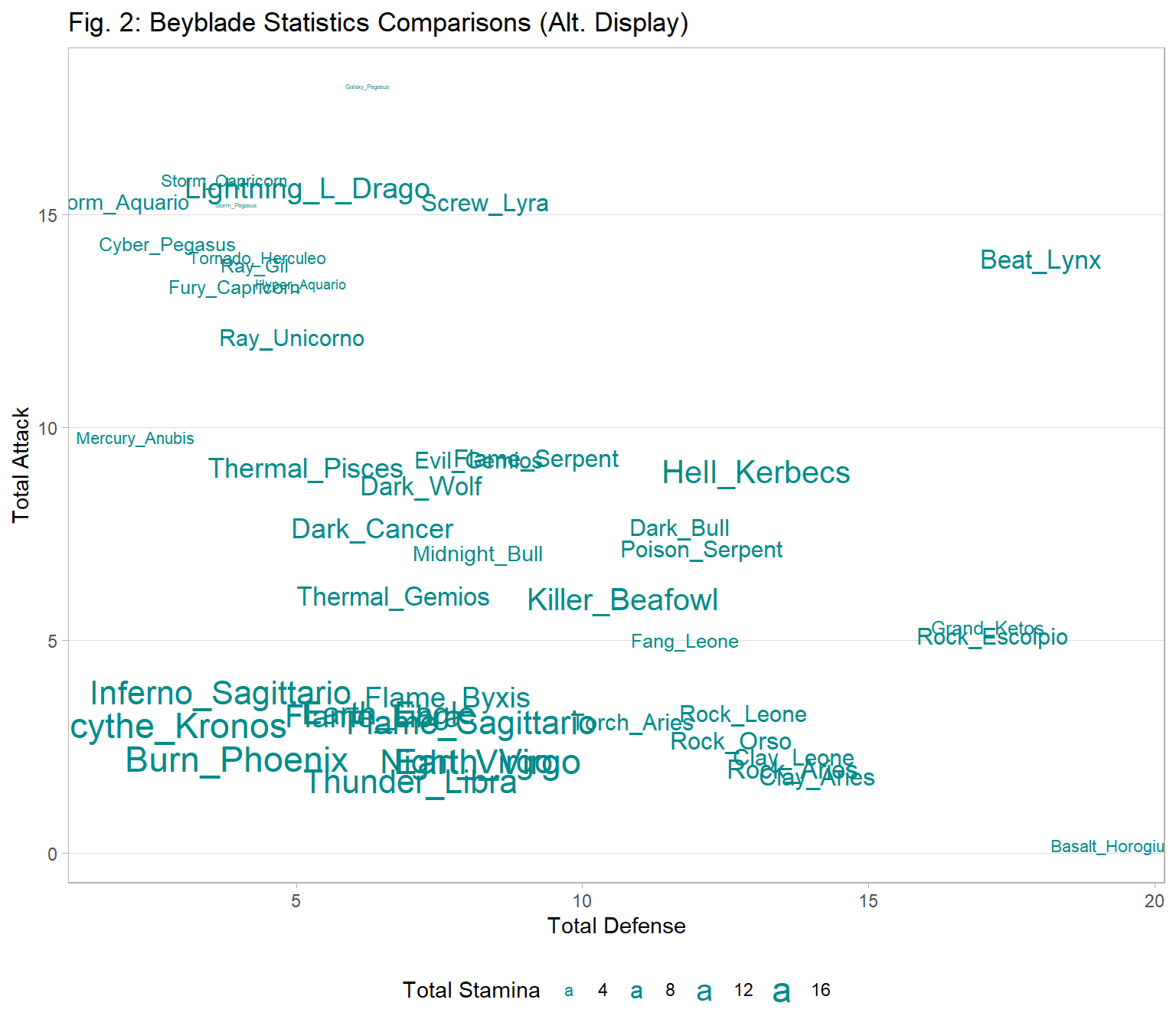

Based on Figure 2, Beat Lynx may be the optimal beyblade among all other Metal Fight beyblades: it has high attack and defense while boasting a moderately high stamina. In other words, although it does not beat Burn Phoenix in terms of stamina, it is an outlier in the generally negative trend between Attack and Defense.

Conclusion

Using rvest to scrape the websites, purrr for iterations, flextable for table formatting, and ggplot2 for plotting (among others), I have employed data science methods to generalize the patterns among the beyblade traits. I have determined that Attack is negatively related to Defense and Stamina, while Defense seemingly is not correlated with Stamina. Overall, the beyblade Beat Lynx is an outlier in that it boasts a high attack and defense while maintaining a moderately high stamina. As such, if the statistics are to be trusted, the optimal beyblade would be Beat Lynx on average among those in Metal Fight.

However, regardless of your own interest in the Beyblade universe, I hope that this post motivates you to (1) learn more about web mining and (2) investigate your favorite franchises with data science. Feel free to expand upon the code presented here–I would love to know what you produce!