Preface
The contents of this blog post originate from the PDF version (https://github.com/robertschnitman/RS_Reports/blob/master/Polls/Sachse/sachse2020.pdf) and its GitBook equivalent (https://rs-sachse2020.netlify.com/).
EDIT 2020-03-27: This post has been updated to use flextable instead of kableExtra to produce a cleaner table for HTML. The PDF and Gitbook reports use the latter, as it is better for PDFs.
Introduction
The purpose of this document is to demonstrate the utility of using the R programming language in reporting polls by walking through the process via the software itself. To showcase its benefits, I use the results of the Sachse, TX January 2020 Special Election (pre-runoff). Ultimately, the advantages are (1) automated reporting, (2) visualizations, and (3) clean presentations of the results.
Setup
Loading Libraries
The following R libraries are used in this report–please install them to be able to replicate the sections that follow. The tidyverse library is a metapackage–a package containing other packages–consisting of useful data management and visualization tools (https://www.tidyverse.org/). The library magrittr is used for its pipe operations, which facilitate readable code by being able to “pass” functions to other functions (https://magrittr.tidyverse.org). Finally, the packages knitr and flextable are used to present formatted tables (https://github.com/yihui/knitr) (https://davidgohel.github.io/flextable/).
R Code: Libaries Loading Loop
# Libraries to use.
libs <- c('tidyverse', 'magrittr', 'knitr', 'flextable')

# For each library...
for (i in libs) {

  # If it's not already installed...
  if (!require(i, character.only = TRUE)) {

    # Install it...
    install.packages(i)

    # Then load it.
    library(i, character.only = TRUE)

  }

}
Data
The polling data were obtained on February 20, 2020 from the City of Sachse TX government website (https://www.cityofsachse.com/365/Election-Results) (See Figure 1 below).
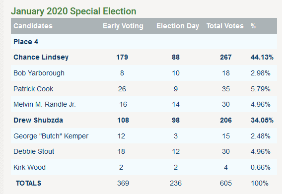
Figure 1: Sachse, TX January 2020 Special Election Results (Pre-runoff)
Importing the Data
The polling results are copied to a comma-separated values (CSV) file named sachse2020.csv and imported via the read_csv() function, presenting the results with the flextable() function to produce a formatted table.
R Code: Importing the Dataset and Presenting the Results in a Tabular Format
data <- read_csv('sachse2020.csv')

data %>%
  arrange(desc(votes_total_pct)) %>%
  set_names(c('Candidate', 'Early Voting', 'Election Day',
              'Total Votes', 'Total Votes %')) %>%
  flextable() %>%
  set_caption(caption = 'Table 1: Special Election Results (Pre-runoff)') %>%
  footnote(part = 'header',
           value = as_paragraph('Source: https://www.cityofsachse.com/365/Election-Results')) %>%
autofit()Candidate1 | Early Voting1 | Election Day1 | Total Votes1 | Total Votes %1 |
Chance Lindsey | 179 | 88 | 267 | 44.13 |
Drew Shubzda | 108 | 98 | 206 | 34.05 |
Patrick Cook | 26 | 9 | 35 | 5.79 |
Melvin M. Randle Jr. | 16 | 14 | 30 | 4.96 |
Debbie Stout | 18 | 12 | 30 | 4.96 |
Bob Yarborough | 8 | 10 | 18 | 2.98 |
George "Butch" Kemper | 12 | 3 | 15 | 2.48 |
Kirk Wood | 2 | 2 | 4 | 0.66 |
1Source: https://www.cityofsachse.com/365/Election-Results | ||||
Graphing the Results
To easily visualize the poll rankings, we plot a bar chart of the total votes by candidate using ggplot2 functions, arranging the bars by total votes in descending order with the reorder() function. The graph places the candidates on the vertical axis so that their names are more easily readable than if they were on the other axis. Percentages are displayed so that readers may know the relative magnitude of the total votes.
R Code: Graphing the Total Votes by Candidate
ggplot(data) +
  aes(x = reorder(candidate, votes_total),
      y = votes_total,
      fill = reorder(candidate, votes_total),
      label = paste0(votes_total,'; ', votes_total_pct, '%')) +
  geom_bar(stat = 'identity') +
  geom_text(nudge_y = 36) +
  scale_fill_brewer(palette = 'Blues') +
  ylim(0, 350) +
  coord_flip() +
  labs(x = '',
       y = 'Total Votes',
       title = 'Figure 2: Total Votes by Candidate') +
  theme_light() +
  theme(panel.grid.minor = element_blank(),
        panel.grid.major.y = element_blank(),
        legend.position = 'none')
For the next graph, early voting numbers are plotted against Election Day votes to grasp their relationship more clearly. First, a function called theme_light2()–based on theme_light from ggplot2–is created in a way that emphasizes the data points by minimizing the number of non-data elements (e.g. background color).
R Code: Theme Function
theme_light2 <- function() {

  theme_light() +
  theme(panel.grid.minor = element_blank(),
        panel.grid.major.x = element_blank(),
        legend.position = 'none')

}
To plot the names of the candidates more easily, we extract only their last names with a combination of gsub() from base R; str_split() from the stringr library within tidyverse; and map_chr() from the purrr package within tidyverse. A plot with text as the geometry is then plotted.
R Code: Graphing Early Voting and Election Day Votes
data$last_name <- data$candidate %>%
  gsub(' Jr\\.', '', .) %>%
  str_split(' ') %>%
  map_chr(~ .x[length(.x)])

ggplot(data) +
  aes(x = votes_early, y = votes_election_day, label = last_name) +
  geom_text(col = 'cyan4', position = position_jitter()) +
  labs(y = 'Votes on Election Day',
       x = 'Votes During the Early Voting Period',
       title = 'Figure 3: Early and Election Day Voting Behavior')  +
  theme_light2()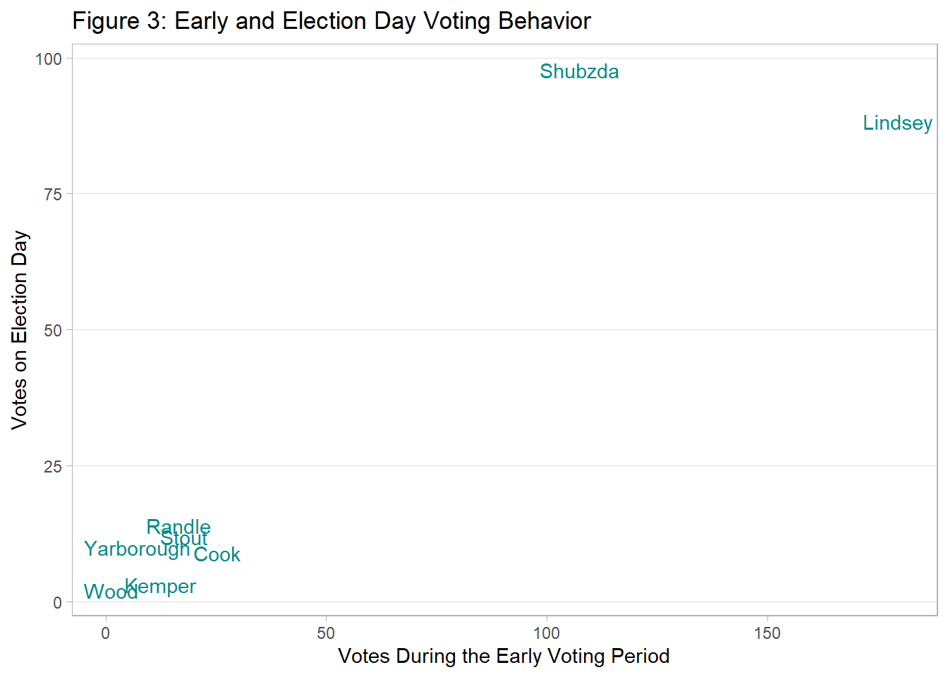
Conclusion
As shown, the advantages of using the R programming language in reporting polls are (1) automated reporting, (2) visualizations, and (3) clean presentations of the election results. Because the code is reusable, the likelihood of human-made errors lower than if the information were to be generated manually. Adding visualizations allow readers to summarize the table information of the results, as well as the ability to examine other kinds of relationships beyond a simple table of results. Finally, these results may be cleanly presented through the use of external packages.
Limitations
One limitation of this work is that the dataset must be in a CSV format. Second, the dataset must be arranged such that there are five required columns: “Candidate,” “Early Voting,” “Election Day”, “Total Votes,” and “Total Votes %.” Third, it assumes that the link to the election results are fixed (i.e. does not change). Finally, some users may feel daunted by the amount of setup and programming required.
Future Work
In the future, this document will serve as a proof-of-concept for a web application via R Shiny in which users can upload polling results and said application would produce a basic written report with tables and graphs.
References
City of Sachse. Election Results; January 2020 Special Election. https://www.cityofsachse.com/365/Election-Results. Accessed 2/20/2020.
Gohel, David. flextable. https://davidgohel.github.io/flextable/. Accessed 3/27/2020.
Magrittr. https://magrittr.tidyverse.org/. Accessed 2/20/2020.
Tidyverse. https://www.tidyverse.org/. Accessed 2/20/2020.
Xie, Yihui. knitr. https://github.com/yihui/knitr. Accessed 2/20/2020.