Using Residuals Percent in OLS Diagnostics

Many students (myself included) were taught to analyze the raw residuals when diagnosing regression models, but not in terms of percent. The benefit of the latter is that we can assess the relative magnitude of error from our regression model.

To display the residuals as a percent (henceforth Residuals, %), let’s first load some necessary libraries.

libs <- c('tidyverse', 'magrittr', 'ggthemes', 'gridExtra')

# For each library, check if they are installed.
## If not, install and load them.
for (i in libs) {
  
  if (!require(i, character.only = TRUE)) {
    
    install.packages(i)
    library(i, character.only = TRUE)
    
  }
  
}

Second, let’s estimate a model and generate the fitted values and residuals. We’ll use the mtcars dataset pre-loaded into R for this example.

# Estimate model.
## mtcars is pre-loaded into R.
mymodel <- lm(mpg ~ wt + hp + gear + am, mtcars)

# Generate fitted and residual values.
fr <- data.frame(fit = predict(mymodel),
                 res = resid(mymodel))

# Residuals as proportions.
fr$res_pct <- with(fr, res/(fit + res))

Third, let’s generate a scatter plot between the residuals percents and the fitted values, as well as a histogram of the former.

# Set up 1x2 plot.
par(mfrow = c(1, 2))

# Scatter plot
with(fr, plot(res_pct ~ fit,
              ylab = 'Residuals, %',
              xlab = 'Fitted Values',
              col  = 'cyan4',
              main = 'Residuals, % vs. Fitted Values'))
abline(h = 0, lty = 2)

# Histogram
hist(fr$res_pct, 
     col  = 'salmon',
     main = 'Distribution of Residuals %',
     xlab = 'Residuals, %')

We can replicate these graphs with ggplot2 graphics.

# Scatter plot
g1 <- ggplot(fr) + 
  aes(y = res_pct, x = fit) + 
  geom_point(col = 'cyan4') + 
  geom_hline(yintercept = 0, linetype = 2) + 
  labs(y = 'Residuals, %',
       x = 'Fitted Values',
       title = 'Residuals, % vs. Fitted Values') + 
  theme_calc() # From ggthemes.

# Histogram
g2 <- ggplot(fr) + 
  aes(x = res_pct) + 
  geom_histogram(col = 'black', 
                 fill = 'salmon',
                 bins = NROW(fr)/2) + 
  labs(x = 'Residuals, %',
       title = 'Distribution of Residuals %') + 
  theme_calc() # From ggthemes.

# Arrange the ggplots in a grid
grid.arrange(g1, g2, ncol = 2, nrow = 1) # From gridExtra.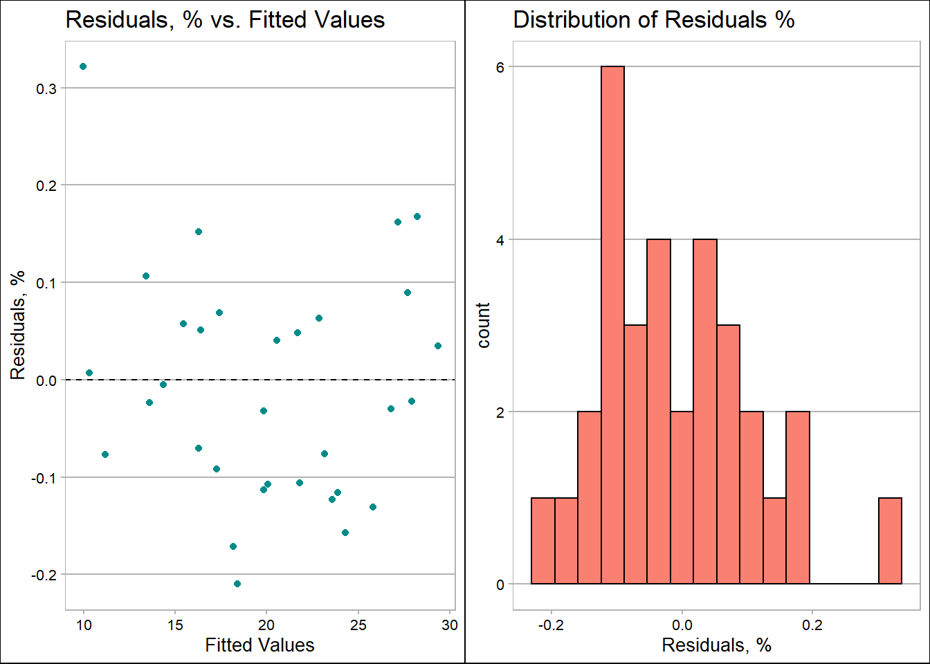

In summary, we have learned how to calculate Residuals, % and graph them with Base R and ggplot2. Try using these techniques the next time you diagnose your models!